I did develop this procedure to find a QSO window in order to maximize my odds to work the Andaman Island 2004 dx-pedition, which was my very last needed country. The results were so good that I did repeat it to work several others dx-peditions. I decided to share it with the ham community, mostly, to the sun venerator guys.
I define QSO window as being the time span when the signals from the major interfering areas are weaker or at maximum equal to mine.
To do that, first of all, I select the potential interfering areas: K6 (Los Angeles), K2 (New York), JA (Tokyo) and I0 (Rome). These areas roughly represent the biggest pile-up generator, however, you may change those areas to fit your needs.
The software
I decided to use the ITSHBC suite for the simplest reason ever: I can use it. Besides of this stupid argument the suite does provide several useful tools, and the most important: it is free of charge. If you are not familiarized with it I do recommend you to stop by at OH6BG site where the VOACAP, one of the components of the ITSHFBC suite, is well explored. Jari, OH6BG, has made a terrific job digging deep for the VOACAP buried treasures.
On the other hand, if you want a simplest approach with the same results you may choose the WINCAP a very nice and well-documented software written by James Tabor, KU5S. He has also written a procedure to achieve the same QSO window. I use either the WINCAP or VOACAP depending upon my state of mind.
You will also need a spreadsheet and chart generator software. I use the MS-Office (TM) suite that does provide all the needed tools.
The very first task is to select the DX station and the date that it expected to show up. To do this tutorial I selected the January 2007 Lakshadweep Island, VU7RG. Of course the results are referred to that date and its solar data as well. At that time the SSN number was 12, so, you will need to replace this value with the current one. Of course you must change the PY2YP location to your own QTH. The next step is selecting the interfering areas, as said above.
After that I define the antennas and power for these areas, which are better or at least equal to mine, and run the circuits setting the DX spot as the target.
Setting up
Select and run the application VOACAP from the ITSHFBC suite, you will have this set up screen:
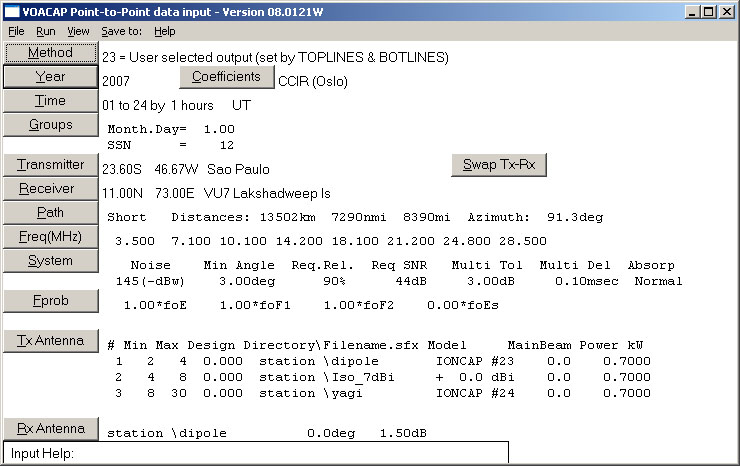
Change the variables accordingly, again I recommend to visit the "Setting VOACAP Input Parameters" page to understand all the parameters meanings. You must be warned with the output power; once the VOACAP is a software written for broadcasting use the output power default is 500 kW, which slightly exceeds our own linear amplifier output :-).
Now, you will need to change the TX antenna settings accordingly to your available antennas

You must change the "Transmitter" field before running all the circuits: your own QTH (PY2YP in this example), K2, K6, JA and I0 before each run.
You also have to configure the antennas running the HFANT application from the ITSHFBC suite:

If you are using a tribander or any kind of shortened antenna you may not find a pre-defined model; in this case I recommend you to select the Type 00 Constant Gain Isotropic and setting up the antenna gain, say, 5 dBi or the best value for your antenna gain. This is not the best solution, but it does workout:

Running the circuits
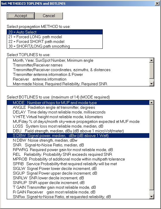
Run the application VOACAP using method 23 which does allow you to select the output parameters:
Running the software you will have an output like this one:
|
1.0
|
9.3
|
3.5
|
7.1
|
10.1
|
14.2
|
18.1
|
21.2
|
24.9
|
28.0
|
30.0
|
Freq
|
|
|
F2F2
|
F2 E
|
F2F2
|
F2F2
|
F2F2
|
F2F2
|
F2F2
|
F2F2
|
F2F2
|
F2F2
|
Mode
|
|
|
-158
|
-187
|
-138
|
-158
|
-184
|
-248
|
-301
|
-326
|
-327
|
-327
|
SDBW
|
In the first line we have: GMT hour, MUF frequency, then the selected frequencies. At the second line we have the propagation mode, which you will need to manually exclude this kind of line in the entire table, there is no way to automatic do this. The third line is what we really need.
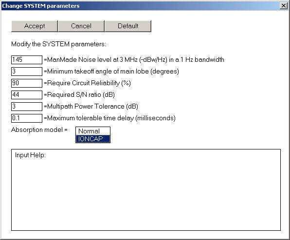
It is a good idea to run the circuit again changing the Absorption Model to IONCAP, under SYSTEM button; this is an older model that, accordingly to some people, it gives better results on lower bands, up to 14 MHz (tnx OH6BG).
Here the work really begins. You will need to work out the reports into an Excel(TM) spreadsheet and then produce the needed graphic.
Save the entire output into a spreadsheet then erase all the mode lines. The final worksheet will look like this:
|
Hour
|
3.5
|
7.1
|
10.1
|
14.2
|
18.1
|
21.2
|
24.9
|
28.0
|
|
1
|
-204
|
-167
|
-173
|
-212
|
-294
|
-334
|
-335
|
-336
|
|
2
|
-227
|
-167
|
-152
|
-172
|
-212
|
-250
|
-298
|
-333
|
|
3
|
-262
|
-174
|
-158
|
-165
|
-212
|
-265
|
-330
|
-331
|
|
4
|
-318
|
-220
|
-165
|
-179
|
-215
|
-282
|
-332
|
-332
|
|
5
|
-408
|
-258
|
-202
|
-182
|
-195
|
-225
|
-277
|
-320
|
|
6
|
-508
|
-305
|
-220
|
-190
|
-204
|
-241
|
-295
|
-339
|
|
7
|
-733
|
-344
|
-236
|
-195
|
-205
|
-256
|
-300
|
-345
|
|
8
|
-893
|
-380
|
-268
|
-182
|
-193
|
-224
|
-256
|
-295
|
|
9
|
-931
|
-368
|
-290
|
-182
|
-170
|
-213
|
-277
|
-353
|
|
10
|
-980
|
-519
|
-297
|
-191
|
-156
|
-173
|
-206
|
-258
|
|
11
|
-976
|
-517
|
-238
|
-191
|
-160
|
-163
|
-198
|
-245
|
|
12
|
-937
|
-501
|
-281
|
-188
|
-161
|
-160
|
-192
|
-242
|
|
13
|
-939
|
-383
|
-280
|
-191
|
-172
|
-155
|
-175
|
-187
|
|
14
|
-875
|
-375
|
-276
|
-184
|
-169
|
-160
|
-167
|
-186
|
|
15
|
-589
|
-364
|
-265
|
-183
|
-168
|
-159
|
-173
|
-181
|
|
16
|
-553
|
-333
|
-245
|
-175
|
-162
|
-161
|
-172
|
-189
|
|
17
|
-464
|
-284
|
-221
|
-168
|
-161
|
-173
|
-186
|
-231
|
|
18
|
-366
|
-244
|
-175
|
-160
|
-164
|
-179
|
-216
|
-282
|
|
19
|
-303
|
-208
|
-165
|
-159
|
-175
|
-201
|
-267
|
-342
|
|
20
|
-259
|
-177
|
-159
|
-167
|
-205
|
-266
|
-335
|
-324
|
|
21
|
-232
|
-169
|
-152
|
-172
|
-233
|
-311
|
-327
|
-327
|
|
22
|
-186
|
-165
|
-155
|
-183
|
-264
|
-339
|
-331
|
-331
|
|
23
|
-192
|
-166
|
-159
|
-207
|
-311
|
-333
|
-334
|
-335
|
|
24
|
-190
|
-165
|
-182
|
-307
|
-331
|
-335
|
-336
|
-337
|
After running the entire prediction you have to careful analyze your best signals at the DX site and elect the bands for the next step. Of course, the chances for working the new one increase when your signals go strong.
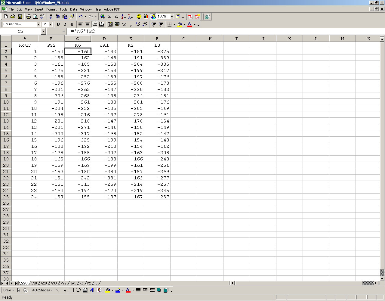
Re-run the VOACAP for each one of the circuits: K2 – VU7, K6 – VU7, JA1 – VU7, I0 – VU7 and, of course, PY2 – VU7 saving their output data to individual worksheets named PY2, K2, K6, JA1 and I0.
The entire spreadsheet will look like this:
Doing the graphics
You must know a little about generating graphics. If you are not skilled on this matter you may ask a hand from your next-door kid. Basically it is a matter of selecting the source for the Y-axis and the series data, so, please take a look at the image below, it will give you some hint:

The QSO window
You will have a graphic just like this one on 30 meters, for example:
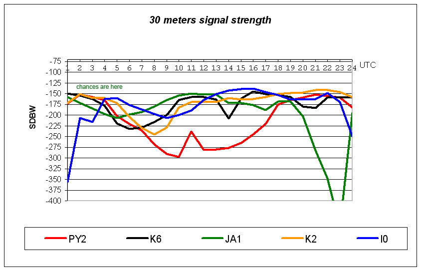
Analyzing the 30 meters graphic the best chance for QSO is between 02:00Z and 04:00Z when my signals in the VU7 site will be close to the K2 guys. Please notice that the PY2 red line is close to the K2 orange line.

On the other hand, the 20 meters band shows the QSO window clearly defined between 17:30Z and 23:30Z, please notice that the PY2 red line is flying alone. If the DX is on the air, you will call only once to be logged :-).
S DBW to S Meter Correlation Table
Jari, OH6BG, offers the S DBW to S Meter correlation table in his site reproduced below:
|
S DBW
|
W (50
Ohm)
|
dBuV
|
microvolts
|
S Meter
|
|
-43.01
|
5.00E-05
|
93.98
|
50000.000
|
S9+60 dB
|
|
-53.01
|
5.00E-06
|
83.98
|
15811.388
|
S9+50 dB
|
|
-63.01
|
5.00E-07
|
73.98
|
5000.000
|
S9+40 dB
|
|
-73.01
|
5.00E-08
|
63.98
|
1581.139
|
S9+30 dB
|
|
-83.01
|
5.00E-09
|
53.98
|
500.000
|
S9+20 dB
|
|
-93.01
|
5.00E-10
|
43.98
|
158.114
|
S9+10 dB
|
|
-103.01
|
5.00E-11
|
33.98
|
50.000
|
S9
|
|
-109.03
|
1.25E-11
|
27.96
|
25.000
|
S8
|
|
-115.05
|
3.13E-12
|
21.94
|
12.500
|
S7
|
|
-121.07
|
7.81E-13
|
15.92
|
6.250
|
S6
|
|
-127.09
|
1.95E-13
|
9.90
|
3.125
|
S5
|
|
-133.11
|
4.88E-14
|
3.88
|
1.563
|
S4
|
|
-139.13
|
1.22E-14
|
-2.14
|
0.781
|
S3
|
|
-145.15
|
3.05E-15
|
-8.16
|
0.391
|
S2
|
|
-151.18
|
7.63E-16
|
-14.19
|
0.195
|
S1
|
Conclusion
I know that this procedure is not so easy and does take a lot of time, however, it works so greatly that I can state that it does worth! I did make available the spreadsheet for downloading and some tips to assist you copying and pasting the output data from the VOACAP. Finally, I'd like to say a big thanks to Gregory R. Hand for his impressive software and to Jari Perkiömäki, OH6BG for his great work exploring all the VOACAP facilities.
Please let me know your impressions and suggestions dropping me an e-mail.